ggplot(df, aes(x = body_mass_g)) +
  geom_histogram(bins = 12) +
  labs(title = "Distribution of Body Mass")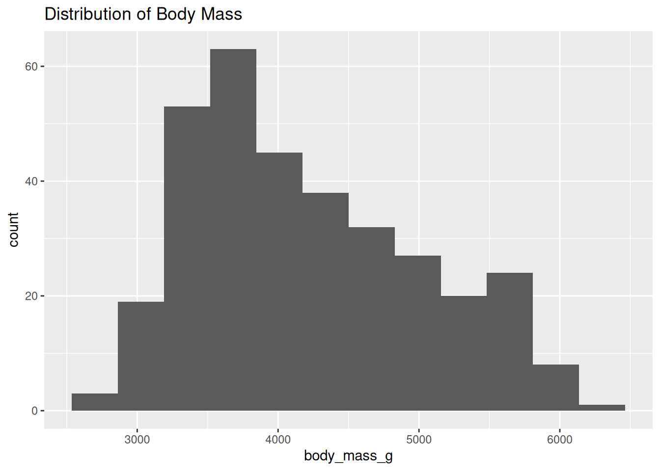
In this section, we begin exploring the cleaned dataset. Exploratory Data Analysis (EDA) helps us understand the structure of the data, identify patterns, and guide our modeling decisions.
EDA is an important step because it allows us to: - understand distributions of variables
- identify relationships between variables
- detect potential outliers or unusual values
- build intuition before fitting models
We start by examining the distribution of body mass to understand its overall shape.
ggplot(df, aes(x = body_mass_g)) +
geom_histogram(bins = 12) +
labs(title = "Distribution of Body Mass")
Next, we explore the relationship between flipper length and body mass.
ggplot(df, aes(x = flipper_length_mm, y = body_mass_g)) +
  geom_point() +
  labs(title = "Body Mass vs Flipper Length")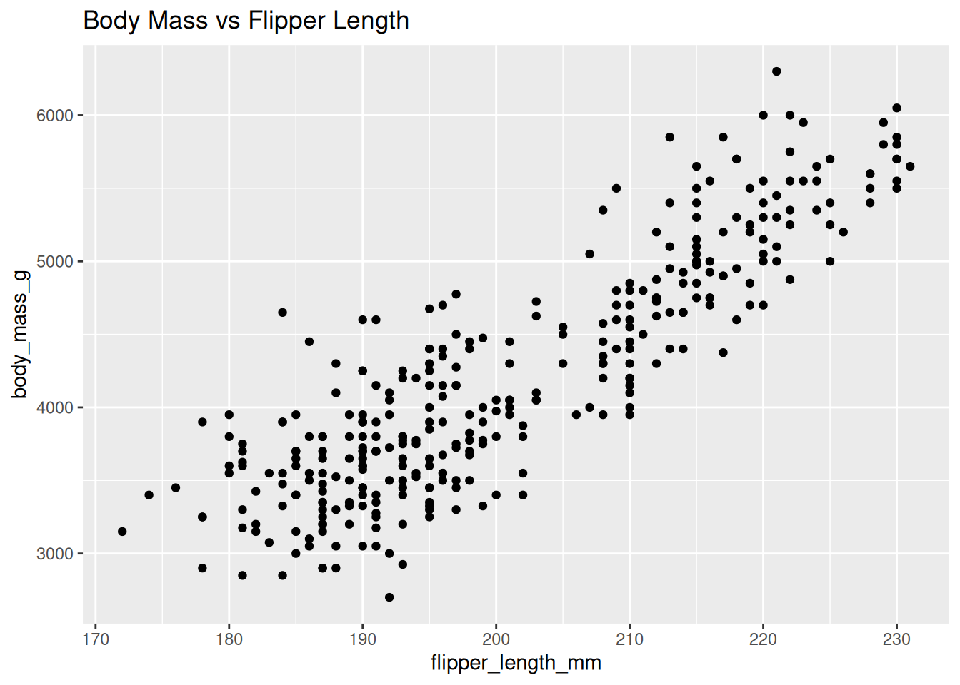
We also examine how bill length relates to body mass.
ggplot(df, aes(x = bill_length_mm, y = body_mass_g)) +
  geom_point() +
  labs(title = "Body Mass vs Bill Length")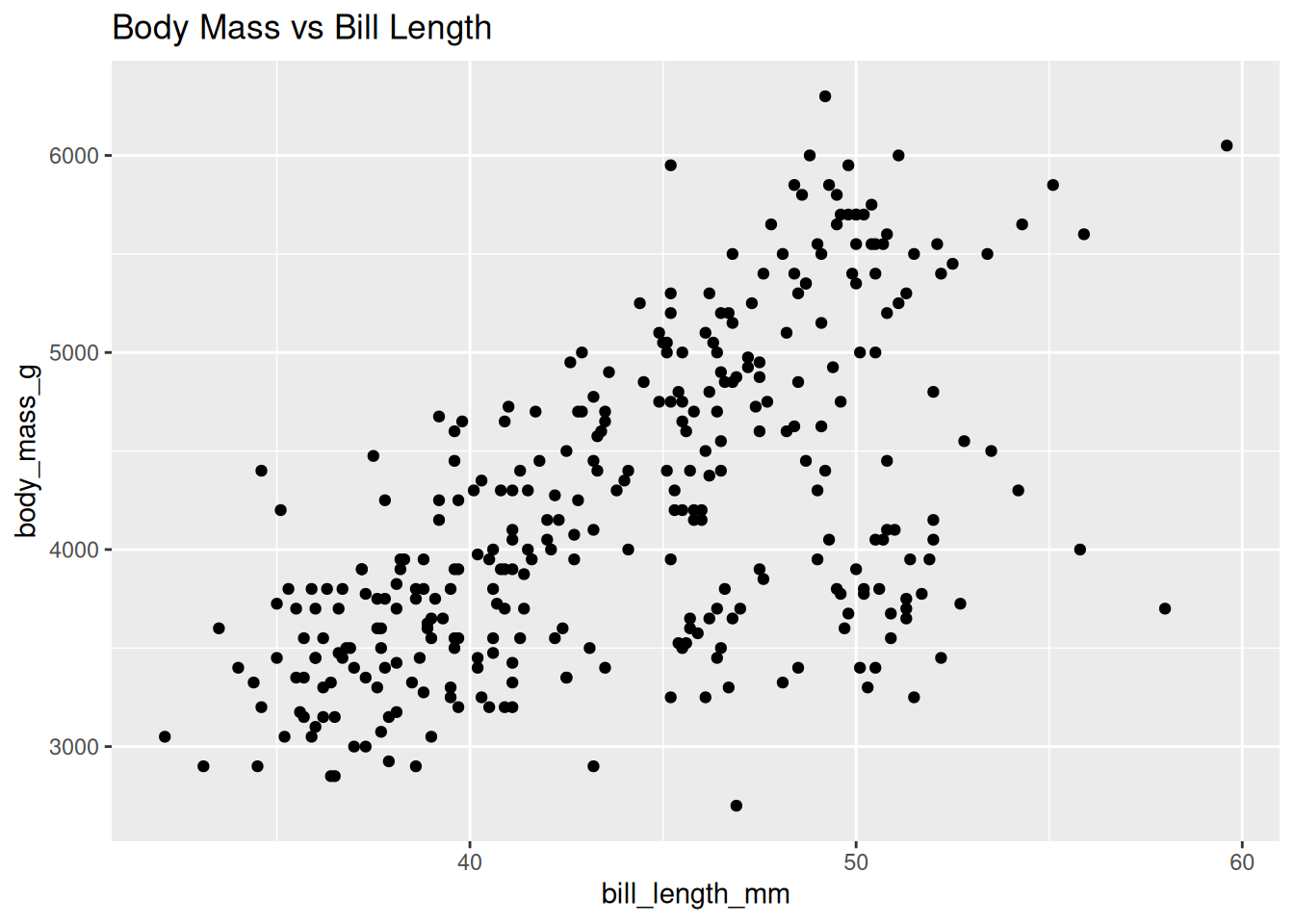
Finally, we compare body mass across different penguin species.
ggplot(df, aes(x = species, y = body_mass_g)) +
  geom_boxplot() +
  labs(title = "Body Mass by Species")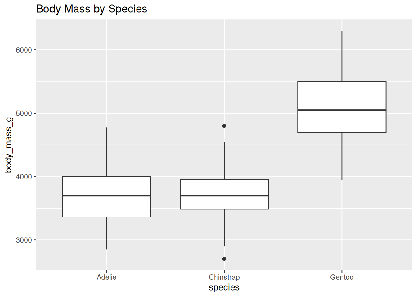
From these plots, we can begin to see patterns in the data:
These insights will guide how we build and interpret our models in the next section.